1. Introduction to 6-DOF Motion Cueing
A 6-DOF (Degrees of Freedom) Stewart platform system simulates movement in six degrees of freedom:
- Translations:
- Sway (side-to-side movement)
- Surge (forward/backward movement)
- Heave (up/down movement)
- Rotations:
- Yaw (rotation around the vertical axis)
- Pitch (rotation around the lateral axis)
- Roll (rotation around the longitudinal axis)
Motion simulation is based on motion cueing, a technique that creates realistic movement sensations by carefully combining high-pass, low-pass, and gain filters. The goal is to simulate acceleration, braking, turns, and turbulence as realistically as possible while staying within the mechanical limits of the platform.
2. Motion Cueing – The First Calculation Step in Motion Simulation
Motion cueing is only the first step in calculating the motion rig’s position in 3D space. Its purpose is to transform acceleration forces generated by the simulation into physical motion, allowing the participant to perceive these forces as realistically as possible.
Limitations of Motion Cueing
A key limitation of motion cueing is that higher G-forces and sustained accelerations cannot be fully simulated. This is because:
- Physical Constraints:
- Servomotor-driven motion platforms can only generate acceleration peaks in the millisecond range, often exceeding 1G for a very brief moment.
- After the initial jerk acceleration, the platform moves toward its target position at a constant speed, which means the participant no longer feels any forces.
- Lack of Sustained Forces:
- In real-world scenarios, sustained G-forces, such as those in high-speed turns or prolonged acceleration, continue to act on the body.
- In a simulator, once the rig reaches its new position, there are no additional forces acting on the participant, making it impossible to simulate long-lasting accelerations accurately.
How Motion Cueing Compensates for These Limitations
- Tilt Coordination: Uses slow rotations (pitch and roll) to trick the inner ear into perceiving a prolonged force.
- High-Frequency Cues: Enhances realism by replicating vibrations and road textures, even if sustained G-forces are absent.
- Washout Filters: Gradually return the rig to its neutral position without noticeable motion, preparing it for the next acceleration phase.
Understanding these fundamental principles and limitations is crucial when fine-tuning motion profiles to achieve the most immersive experience possible within the mechanical constraints of a motion simulator.
2. The Basic Filtering System for 6-DOF Simulations
The filtering system used here works for all types of simulators and provides output as:
- Millimeters for translations
- Degrees for rotations
The system structure is always the same:
- Gain: Amplifies the input value by a given factor. So you transform the incoming force to a movement in mm or degree
- High-pass filter (HPF): Removes slow movements and ensures that the rig returns to the neutral position.
- Low-pass filter (LPF): Smooths out fast movements and reduces jitter.
- Crop operation: Limits values within a predefined range to prevent excessive motion.
2.1. Implementation of Filters for Each Axis
The basic formula for each axis is:
CROP(EMALP(EMALP(EMAHP(GAIN(VALUE; x); y); z); w); min; max)
Where:
- GAIN(VALUE; x): Amplifies the input signal by a factor of x.
- EMAHP(VALUE; y): High-pass filter with cutoff frequency y, removing slow components.
- EMALP(EMALP(VALUE; z); w): Two cascaded low-pass filters with cutoff frequencies z and w, smoothing the motion. each EMALP stands for his own the
- EMALP(VALUE;z)
- CROP(VALUE; min; max): Limits the value within the range min to max.
- GAIN(VALUE, x)
- Purpose: Multiplies the input by a factor x.
- Why: To amplify or attenuate the signal.
- Example: Input = 10, x = 2 → Result = 20.
- EMAHP(VALUE, y)
- Purpose: High-pass filter to remove slow changes.
- Why: Eliminates drift and slow variations.
- Example: Slow rise from 10 to 12 → Result = 0.
- EMALP(VALUE, z) and EMALP(VALUE, w)
- Purpose: Low-pass filters to smooth rapid fluctuations.
- Why: Stabilizes the signal.
- Example: Rapid fluctuations between 10 and 15 → Stabilizes around 12.
- CROP(VALUE, min, max)
- Purpose: Limits the output within min and max.
- Why: Ensures the output stays within acceptable bounds.
- Example: Result = 25, max = 20 → Output = 20.
https://www.youtube.com/channel/UCi4XXEv-mU8aiN9GgKyFx2w/videos
check out the videos for LP in this YT channel
2.1.1. Filter Settings for Translations
Translations require double low-pass filters to smooth motion:
- Sway: CROP(EMALP(EMALP(EMAHP(GAIN(VALUE;5);2000);100);100);-100;100)
- Surge: CROP(EMALP(EMALP(EMAHP(GAIN(VALUE;5);2000);100);100);-100;100)
- Heave: CROP(EMALP(EMALP(EMAHP(GAIN(VALUE;5);2000);100);100);-100;100)
2.1.2. Filter Settings for Rotations
Rotational movements require only one low-pass filter as they produce less jitter:
- Yaw: CROP(EMALP(EMAHP(GAIN(VALUE;0.3);2000);100);-5;5)
- Roll: CROP(EMALP(EMAHP(GAIN(VALUE;0.3);2000);100);-5;5)
- Pitch: CROP(EMALP(EMAHP(GAIN(VALUE;0.3);2000);100);-5;5)
3. Tilt Coordination – Extending to Additional Degrees of Freedom
In addition to the six main degrees of freedom, the platform can use Tilt Coordination. This method simulates sway and surge accelerations through a slow tilt (roll or pitch) to create a longer-lasting acceleration effect.
- Sway in Roll: CROP(EMALP(EMALP(EMALP(GAIN(VALUE;1);2000);100);100);-5;5)
- Surge in Pitch: CROP(EMALP(EMALP(EMALP(GAIN(VALUE;1);2000);100);100);-5;5)
Explanation:
- Sway in Roll: A lateral tilt can simulate a sustained lateral force.
- Surge in Pitch: A forward/backward tilt can simulate sustained longitudinal acceleration.
3.1. Importance of Tilt Coordination
Tilt coordination is used in flight simulators and racing simulations to simulate long-duration forces that would otherwise be impossible to represent within the platform’s physical limitations.
4. Fine-Tuning the Motion Profile
4.1. Adjusting Gain Values
- Increase Gain (amplification factor) for each axis to enhance movements.
- Typical values for translations: 3 to 10.
- Typical values for rotations: 0.3 to 1.
4.2. Adjusting the Low-Pass Filters
- Higher values (200, 300, 400, 500) = Smoother and more gradual movements.
- Lower values (50, 80) = More detailed and responsive motion.
4.3. High-Pass Filter for Returning to Neutral Position
- Large rigs can use high values like 3000 or 4000 for gradual return.
- Smaller rigs require lower values for a faster reset.
By fine-tuning the gain and filter values, users can adjust the motion profile to achieve an optimal balance between realism and comfort.
This system works for all simulators, whether flight, racing, or general driving simulations.
5. Motion Cueing Software
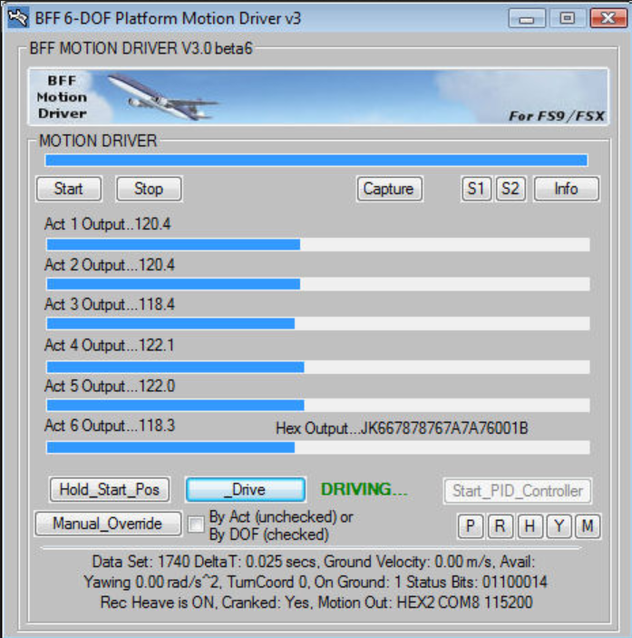
IAN BFF Simulation
6dof Motion cueing Software
FLYPT Mover
best 6dof motion cueing software
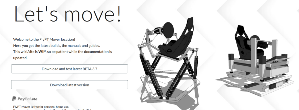
This is the most complex and highly adjustable software for 6DOF motion cueing and motion cueing in general. With wide support for simulation and software, it is highly recommended for those who operate do-it-yourself rigs.
Motion4Sim Dashboard integrated Motionsystem
integrated 6dof Motion cueing System for Motions4sim controllers

Dashboard Motion was developed to provide users with easier access to motion tuning systems. The profiles can be fine-tuned using sliders, and the system automatically connects to loaded simulations when they are online.